Why Qwerty? #

General-purpose quantum programming languages today (e.g., Qiskit, Q#, or Quipper) are gate-oriented.

For example, consider the Bernstein–Vazirani algorithm, which determines a secret string \(s\) given a black box (“oracle”) that computes \(f(x) = x_1s_1 \oplus x_2s_2 \oplus \cdots \oplus x_ns_n\) . The code for Bernstein–Vazirani could look like the following:

Q# (source)

 1use queryRegister = Qubit[n];
 2use target = Qubit();
 3
 4X(target);
 5H(target);
 6
 7within {
 8    ApplyToEachA(H, queryRegister);
 9} apply {
10    Uf(queryRegister, target);
11}
12
13let resultArray = ForEach(MResetZ, queryRegister);
14Reset(target);
15return resultArray;

Qwerty

1return '+'[N] | f.phase \
2              | pm[N] >> std[N] \
3              | std[N].measure

Notice that the Q# code above is written in terms of quantum gates (e.g., the Pauli X and the Hadamard gate H). Even Uf is expressed as gates (not shown above). Thus, to read and write Q# code, you need a deep understanding of quantum gates.

Instead, the Qwerty code above speaks in term of bases such as pm[N] and std[N]. But how?

Thinking in Bases #

Imagine the typical Cartesian plane with a basis \(\hat{i},\hat{j}\), where \( \hat{i} \triangleq \begin{bmatrix} 1 \\ 0 \end{bmatrix} \) and \( \hat{j} \triangleq \begin{bmatrix} 0 \\ 1 \end{bmatrix} \). By basis, we mean any vector in the 2D plane can be represented as a linear combination of basis vectors, i.e., for any \(\vec{v}\), there exist \(a\) and \(b\) such that \( \vec{v} = a\hat{i} + b\hat{j} \).

The core primitive of Qwerty is a basis translation. Suppose \(\hat{p},\hat{m}\) is another basis. Then a basis translation \(T\) from \(\hat{i},\hat{j}\) to \(\hat{p},\hat{m}\) performs the following:

\[ a\hat{i} + b\hat{j} \\ \Downarrow_T \\ a\hat{p} + b\hat{m}\]

That is, \(a\) and \(b\) are preserved; only the basis changes. Visually, this looks like this:

Above, we define \(\hat{p} \triangleq \frac{1}{\sqrt{2}}(\hat{i} + \hat{j})\) and \(\hat{m} \triangleq \frac{1}{\sqrt{2}}(\hat{i} - \hat{j})\).

It turns out this space is very, very similar to the state space of a qubit. The differences are the following:

For the purposes of bitwise logic, quantum programmers treat \(\hat{i}\) as 0 and \(\hat{j}\) as 1; in Qwerty, you write these as '0' and '1', respectively
In Qwerty, \(\hat{p}\) above is '+' and \(\hat{m}\) is '-'. Both are superpositions of '0' and '1'
The vector space is complex, not real — it’s \(\mathbb{C}^2\) instead of \(\mathbb{R}^2\)
Every qubit state must be a unit vector (i.e., on the thin gray circle above)

In Qwerty, you can write the basis \(\hat{i},\hat{j}\) as {'0','1'}, or std for short. Similar, the plus-minus basis \(\hat{p},\hat{m}\) can be written as {'+','-'} or pm. You’d write the basis translation \(T\) above as std >> pm. (This compiles to the famous Hadamard gate.)

Application: Bernstein–Vazirani #

The Bernstein–Vazirani algorithm originates from a 1993 paper by Ethan Bernstein and Umesh Vazirani, where the authors used it to make a complexity theory argument for the power of quantum computers. Specifically, a classical algorithm will need \( N \) queries to the black box for \( f(x) \) to determine the secret string \(s\), whereas the quantum algorithm needs only \( 1 \).

Algorithm Intuition #

The black box for \(f(x)\) has a remarkable property: when applied to a quantum register of qubits in the '+' state (a superposition of 0 and 1), the black box will flip each '+' state to a '-' state (another superposition orthogonal to '+') when there is a 1 in the secret string at that position. This gives rise to the procedure drawn below:

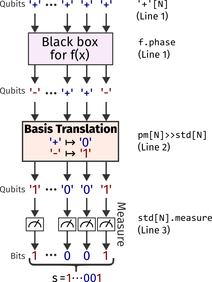
The line numbers are the line numbers in the Qwerty code snippet above. The step that reveals the answer is the basis translation from the '+'/'-' basis (“pm”) to the standard '0'/'1' basis (“std”). The Qwerty syntax pm[N] >> std[N] is this operation in parallel on \(N\) qubits.

Technical Algorithm Details

If you are familiar with typical notation for quantum algorithms, here is the math for Bernstein–Vazirani. If the oracle is defined as \( U_f\vert x \rangle \mapsto (-1)^{x \cdot s}\vert x \rangle \), where \( x \cdot s \) is bitwise dot product mod 2, then the algorithm proceeds as follows:

\[\begin{aligned} \vert+\rangle^{\otimes n} ={}& \frac{1}{\sqrt{2^n}}\sum_{x \in \{0,1\}^n} \vert x\rangle \\ \xrightarrow{(1)}{}& \frac{1}{\sqrt{2^n}}\sum_{x \in \{0,1\}^n} (-1)^{f(x)}\vert x\rangle \\ ={}& \frac{1}{\sqrt{2^n}}\sum_{x \in \{0,1\}^n} (-1)^{x \cdot s}\vert x\rangle \\ ={}& \frac{1}{\sqrt{2^n}}\left(\vert 0 \rangle + (-1)^{s_1}\vert 1 \rangle \right) \\ & \qquad\otimes\left(\vert 0 \rangle + (-1)^{s_2}\vert 1 \rangle \right) \\ & \qquad\otimes\cdots\otimes\left(\vert 0 \rangle + (-1)^{s_n}\vert 1 \rangle \right) \\ \xrightarrow{(2)}{}& \vert s_1 \rangle \otimes \vert s_2 \rangle \otimes \cdots \otimes \vert s_n \rangle \\ \xrightarrow{(3)}{}& s \end{aligned}\]

The numbers on the steps (arrows) above correspond exactly to the line numbers of the Qwerty code above. These steps are:

Apply the black-box oracle for \( f(x) \)
Perform a basis translation from \( \vert + \rangle / \vert - \rangle \) to \( \vert 0 \rangle / \vert 1 \rangle \).
Measure in the standard (\( \vert 0 \rangle / \vert 1 \rangle \)) basis

Revisiting the Qwerty Code #

The Qwerty code above prepares \(N\) qubits in the '+' state on the start of line 1. The qubits then flow left-to-right through the following operations (think of | like a Unix shell pipe):

A classical instantiation of \(f(x)\) using the syntax f.phase. This synthesizes f such that applying f.phase to e.g. '1011' yields -'1011' (a scalar factor of \(-1\)) if \(f(1011) = 1\) else the state remains '1011'.
A basis translation from the \(N\)-qubit pm basis to the \(N\)-qubit std basis, written as pm[N] >> std[N] on line 2.
A measurement in the \(N\)-qubit std basis on line 3, yielding \(N\) classical bits.

We believe these algorithmic steps are far clearer in the Qwerty code above versus the corresponding Q# code. This applies to more than just Bernstein–Vazirani — you can find more examples of Qwerty on the Examples page.